The Discreet Wavelet Transform
Andreas Jönsson, May 2002

The purpose of the Wavelet Transform (WT) is to separate a signal into its frequency components. This is much like the Fourier Transform (FT). The difference is that with the WT we also get the variation of the frequency component over the time. For example, we have a signal that have a high frequency component in the first half. With FT we can see that this frequency component is there but not where it is. With WT we get to see not only that the frequency component is there but also that it is in the first half.

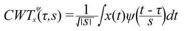
The WT works by repeatedly filtering the signal with a short wave, the wavelet, at different scales and positions. Changing the scale of the wavelet changes the frequency band that is analyzed and the position of the wavelet changes the time frame analyzed. Doing this filtering for every possible scale and position of the wavelet is called the Continuous Wavelet Transform (CWT), and as you can imagine this is a very costly procedure. Fortunately it is not needed to do a complete CWT. After all, low frequencies don't change very fast, thus we will get a good understanding about the frequency component even if we don't measure it very often.

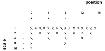
A good scheme to follow when choosing the scales and positions for the wavelet is the dyadic scheme. The dyadic scheme works with multiples of 2. Increase the scale each step multiplying with 2. The position should be increased in steps equal to the scale, e.g. when scale is 1 the position is increased in steps of 1, when scale is 4 position is in steps of 4. Here´s an image that shows the values for the scale and position.

A direct implemenation of this requires the same amount of computions for each step in the scale, we do half the number of filtrations, but the length of the filter is doubled for each step. For those that don't know yet, a numerical filtration involves a component wise multiplication of two arrays. Thus if the filter is of length N, we will need N multiplications.

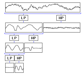
Fortunately this can be heavily optimized by using Nyquist's theorem. Nyquist's theorem says that a sampled signal can't represent signals with frequencies higher than half the sample rate. Because of this we need only make a filtration for every second sample. And by doing a low pass filtering of the signal before doubling the scale, we can remove half the samples of signal since they are redundant anyway. In the second step we will thus have a signal of half its previous length, which is the same as doubling the scale of the filter. This is why the low-pass filter is also known as the scaling filter. I have simplified it immensely but this is basically what is done in the Discreet Wavelet Transform (DWT). For each iteration the signal is filtered with the wavelet and then low-pass filtered and subsampled for the next iteration.

Here is an image that shows what is going on:

The wavelet and scaling filter must be chosen carefully in order to not loose information when computing the transform. If they are chosen correctly the original signal can be rebuilt from the transformed values. I will not go through how the filters should be constructed/chosen here as it is not necessary for understanding wavelet transforms, suffice to say that the filters must be orthogonal to each other so that they split the information in two parts without overlap. The sum of the scaling filter should also equal sqrt(2) in order to keep the energy of the wavelet constant for each level. Here are two examples of such wavelet/scaling filter pairs.

Haar
wavelet	scale
Daubechies
wavelet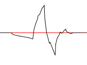	scale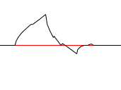

Ones you have chosen the wavelet and scaling filters you compute the DWT like this.

  for( n = 0; n < N/2; n++ )
  {
    yh[n] = x[2n+0]*g[3] + x[2n+1]*g[2] + x[2n+2]*g[1] + x[2n+3]*g[0];
    yl[n] = x[2n+0]*h[3] + x[2n+1]*h[2] + x[2n+2]*h[1] + x[2n+3]*h[0];
  }

N is the length of the input signal. g is the wavelet filter, h the scaling filter, x the input signal and yh the wavelet coefficients and yl the lowpass filtered signal to be used in the next iteration. yh and yl both have half the length of x. Of course, the filters don't have to have lengths of 4, they can have any length you want as long as it is at least 2 values.

The reconstruction can then be made like this.

  for( n = 0; n < N/2; n++ )
  {
    x[2n  ] = yl[n-1]*h[1] + yl[n]*h[3] + yh[n-1]*g[1] + yh[n]*g[3];
    x[2n+1] = yl[n-1]*h[0] + yl[n]*h[2] + yh[n-1]*g[0] + yh[n]*g[2];
  }

yl and yh are the values computed from the DWT. g and h are the exact same filters as in the DWT. If the filters have been chosen properly then x will be reconstructed without any modifications.

Note that the arrays in these examples are not your ordinary arrays. These are circular arrays, which means that the end connects to the start, or in other words indices should be wrapped so that they are always within the bounds of the array. If you don't use circular arrays you will loose some data in the beginning of the signal and will get some errors when reconstructing the signal. This can be solved by padding the signal with zeroes but it is easier to use circular arrays.

To make it easier to understand what is going on, here is an example transform of a signal with length 8. The transform has been written as a matrix multiplication in order to easier show the wrapping of the signal.

  [yl0] = [h3 h2 h1 h0            ][x0]
  [yl1] = [      h3 h2 h1 h0      ][x1]
  [yl2] = [            h3 h2 h1 h0][x2]
  [yl3] = [h1 h0             h3 h2][x3]
  [yh0] = [g3 g2 g1 g0            ][x4]
  [yh1] = [      g3 g2 g1 g0      ][x5]
  [yh2] = [            g3 g2 g1 g0][x6]
  [yh3] = [g1 g0             g3 g2][x7]

To go back we invert the matrix and multiply again.

  [x0] = [h3       h1 g3       g1][yl0]
  [x1] = [h2       h0 g2       g0][yl1]
  [x2] = [h1 h3       g1 g3      ][yl2]
  [x3] = [h0 h2       g0 g2      ][yl3]
  [x4] = [   h1 h3       g1 g3   ][yh0]
  [x5] = [   h0 h2       g0 g2   ][yh1]
  [x6] = [      h1 h3       g1 g3][yh2]
  [x7] = [      h0 h2       g0 g2][yh3]

Note that these examples only show one iteration of the DWT. You should do the transforms recursively on the low-pass filtered values until you only have 1 more value.

Because of the subsampling at each step there will be the exact same amount of data after the transform as before. Commonly this data is stored in a single array with the lowest level of filtered data first, i.e. the data that was computed last comes first. The last half of this array will then contain the highest frequencies in the original signal.

Conclusion

Hopefully you have gotten an understanding of how wavelet transforms work and how they can be implemented. I haven't told you what wavelet transforms are good for, but I'm sure you have heard at least something about them. The most commonly uses are data compression and signal processing. A simple compression scheme would be to transform the signal and then run-length encode the zeroes. In a scheme like this the wavelet should be chosen to give the most zeroes.

If you have some questions or comments about the article you are welcome to e-mail me about them. Also, don't forget to check out the demo with source code that you can download from my site.

Further reading

The Wavelet Tutorial, by Robi Polikar
Wavelet Theory, pdf document from the site of Czech Technical University in Prague